ROC curves for A/B tests?

This question might be a little out there; nevertheless, I wanted to share my thoughts on this topic. It came to my mind after reading about the connection between the $U$ statistic (from the Mann-Whitney $U$ test) and the AUC of the empirical ROC curve estimate (in case you haven’t heard about this relationship, don’t worry, I will explain it in a bit). The former one is frequently used for the evaluation of A/B tests, the latter for summarizing the performance of classification procedures. This blog post will not be about A/B tests nor classification procedures themselves. I assume you are familiar with these concepts already, if not, you might want to read about these topics first, and then continue with this article.

Even though A/B tests and classification problems are different by nature, they also have something in common. In both situation we are dealing with two groups that should be different with respect to a selected feature. And as it seems now, we are even using equivalent statistics for analyzing both of them, the $U$ statistic and the AUC. So what is the difference and why aren’t we using ROC curves for A/B tests as well? There is a good reason for it!

The answer might be obvious for you, but if not you should read this blog post. You never know what tricky questions might be waiting for you in your next job interview

But first things first, let’s briefly recall the definition of ROC curves and some of their properties.

Receiver operating characteristic (ROC) curves are graphical representations of the relationship between the true positive rate (TPR) and the false positive rate (FPR) for all possible threshold values of a binary classifier. They are used to assess the discrimination ability of a classifier and to compare a group of classifiers with each other. Typically, ROC curves are constructed by plotting all (FPR, TPR) points based on the predicted scores on a validation dataset. Afterwards, linear interpolation is applied to connect the points to a curve (see Figure 1 A). This can be seen as a descriptive statistics approach, where only the data at hand is being summarized. On the other side, if we assume the data to be a sample from a population, we can apply statistical inference methods to estimate the real underlying ROC curve (see Figure 1
B). There are many different methods and models described in literature; for a small overview see de Zea Bermudez, Gonçalves, Oliveira & Subtil (2014).

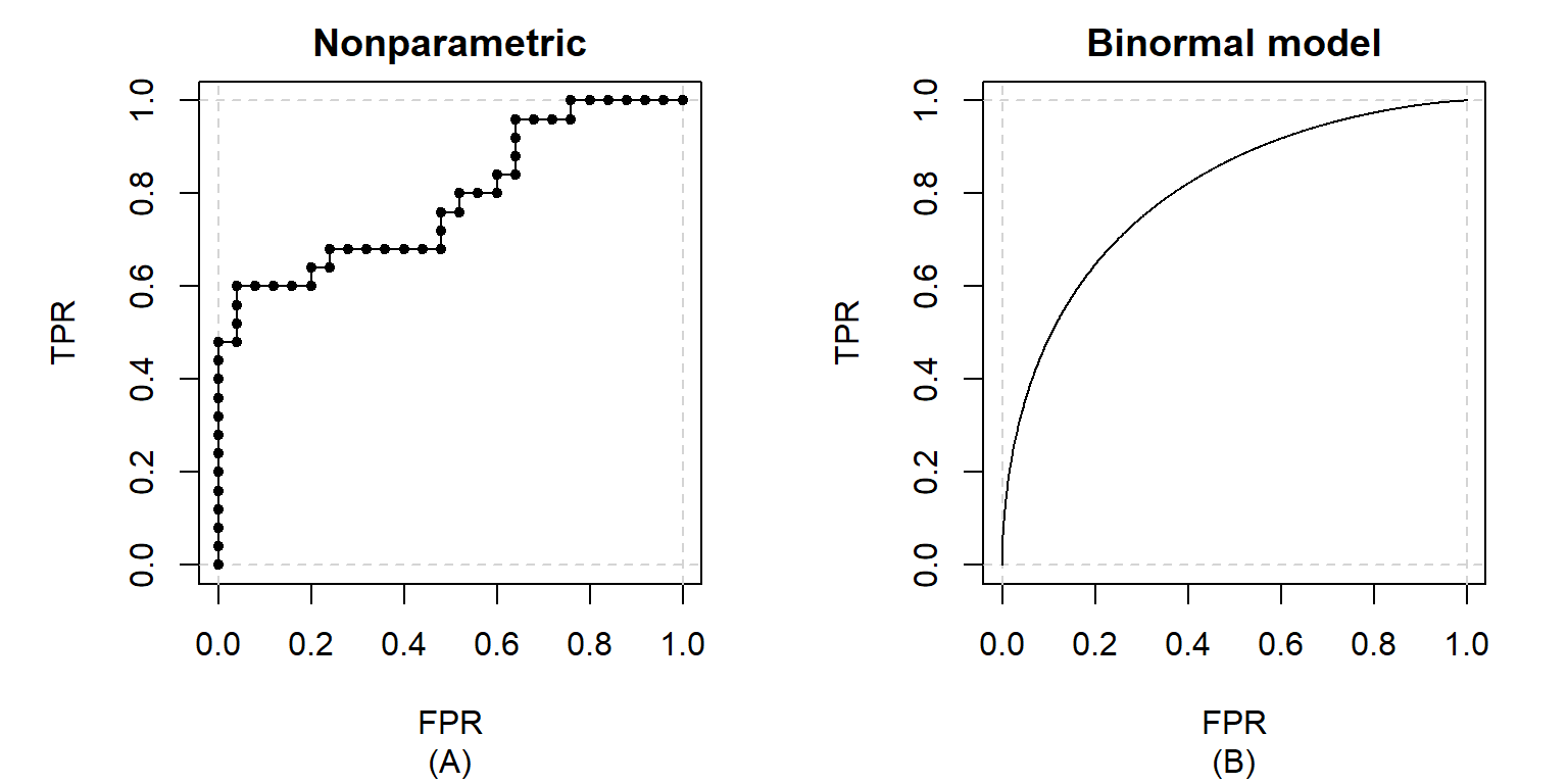
Figure 1: Examples of ROC curve estimates using a nonparametric approach (A) and a binormal model (B)

 

It’s common practice to use summary measures for comparing ROC curves (curve estimates). The probably most widely used one is the area under the curve (AUC). Let’s assume that the scores assigned by our classification procedure to positive and negative entities are realizations of two continuous random variables $X$ and $Y$ , respectively. It can be shown that the theoretical AUC is equal to $P(X>Y)$ , the probability that the score of a randomly chosen positive entity will be higher than the score of a randomly chosen negative one. This should make it clear why an AUC close to 1 is desirable for a classifier.

What do ROC curves have in common with the $U$ statistic?

This becomes quite obvious once you have a closer look at the definition of the $U$ statistic:

$$U=\underset{i=1}{\overset{m}{\sum }}\underset{j=1}{\overset{n}{\sum }}S(X_i,Y_j),$$
where
$$S(X,Y)=\{\begin{array}{ll}1,& \text{if }X>Y\\ \frac{1}{2},& \text{if }X=Y\\ 0,& \text{if }X<Y\end{array}.$$

It’s pretty intuitive that $\frac{U}{mn}$ is a valid estimate of $P(X>Y)$ . But so is the AUC of an estimated ROC curve. In the special case of an empirical estimate (like in Figure 1 A), both methods are equivalent:

$$\begin{array}{}\text{(1)}& \widehat{AUC}=\frac{U}{mn}.\end{array}$$

Does it mean we can use ROC curves for A/B test evaluations?

Not really. We could calculate the ROC curve for an imaginary classifier that would try to assign a user to group A or B based on a selected KPI, but it wouldn’t be very informative for us. The reason for this is that we put emphasis on different things while analyzing A/B tests and when analyzing classifying procedures. In an A/B test our main goal is to assess whether the differences between group A and B are statistically significant, even if they are small; how small they can get and still be business relevant is a different question. When analyzing the performance of a classifier we are checking if the differences are big enough to provide discriminative power.

When testing a new feature on your webpage with an A/B test you probably don’t expect the users behavior to change so drastically that you could make accurate predictions to which group, A or B, a random user belonged, based solely on his behavior. The two probability density functions (PDF) of the measured KPI (a score calculated for each user) from group A and B will be rather “close” to each other. Therefore, the AUC of the estimated ROC curve will be close to 0.5 (see Figure 2). To achieve higher AUC values, the PDFs need to be further “away” from
each other (see Figure 3), which is very unlikely to happen in an A/B test.

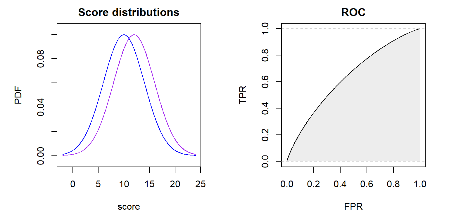
Figure 2: Theoretical PDFs of the scores from positive and negative entities are $\mathcal{N}(12,4^2)$ and $\mathcal{N}(10,4^2)$ , respectively.

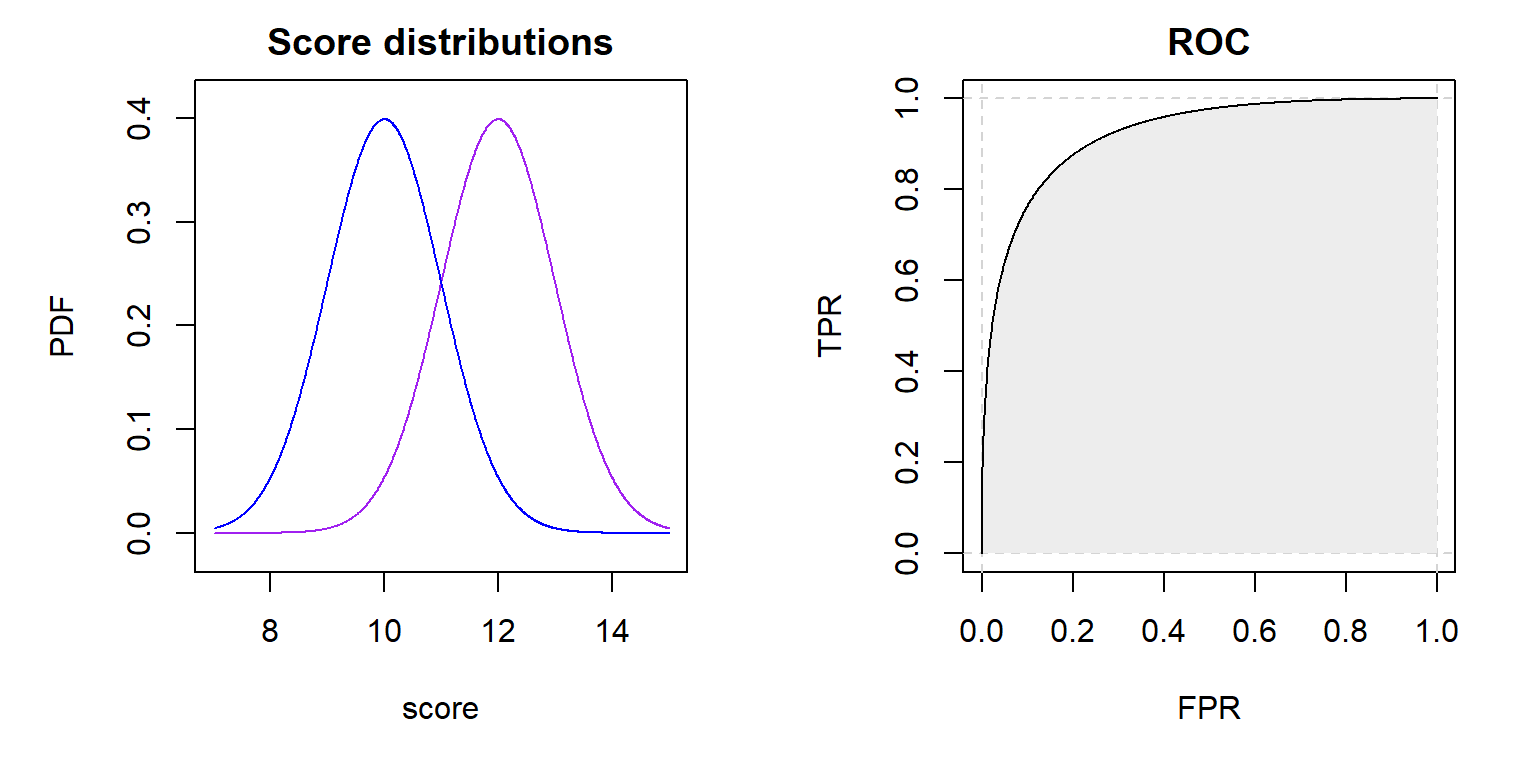
Figure 3: Theoretical PDFs of the scores from positive and negative entities are $\mathcal{N}(12,1^2)$ and $\mathcal{N}(10,1^2)$ , respectively.

How else can we make use of the relationship between the AUC and the $U$ statistic?

A drawback of the Mann-Whitney $U$ test is its computational complexity. For other tests it might be enough to calculate the sample mean and variance, which can be done directly on your DB using performant SQL functions. Not so with this test. Comparing two large samples with the Mann-Whitney $U$ test can get challenging. But luckily in some situation you can use a trick. For example whenever the measure of interest in an A/B test is a simple count (like number of clicks for each user) it’s possible to effectively reduce the data size while keeping all the needed information. It’s enough to count the occurrences of each measure value (e.g. 100 users made 1 click, 200 users made 2 clicks, etc.) in both groups, A and B. This is enough to calculate the $U$ statistic. Unfortunately the standard functions in common statistical software require the raw sample for performing a Mann-Whitney $U$ test. So you have to calculate it yourself… or you can make use of the ROCket package. It provides a set of functions for ROC curve estimation and AUC calculation that can deal with aggregated data. Thanks to the Equation (1), we can also use it to calculate the $U$ statistic.

Imagine you have a dataset of the following form:

#>     clicks user_count group_A group_B
#>  1:      0     905430  453834  451596
#>  2:      1     908886  453605  455281
#>  3:      2     455993  228247  227746
#>  4:      3     151509   75368   76141
#>  5:      4      38192   19021   19171
#>  6:      5       7664    3791    3873
#>  7:      6       1248     596     652
#>  8:      7        190      91      99
#>  9:      8         20      13       7
#> 10:      9          2       1       1

You could create a ROC curve out of it, but most importantly you can calculate the AUC and the $U$ statistic:

prep <- rkt_prep(
  scores = data_agg$clicks, 
  negatives = data_agg$group_A, 
  positives = data_agg$group_B
)
roc <- rkt_roc(prep)
plot(roc)

(AUC <- auc(roc))
#> [1] 0.5009079
(U <- AUC * prep$neg_n * prep$pos_n)
#> [1] 763461645613

The p-value can be now derived using a normal approximation. You can write the necessary code by yourself, but you don’t need to. The development version of ROCket available on GitHub already contains a mwu.test function:

# remotes::install_github("da-zar/ROCket")
mwu.test(prep)
#> 
#>  Mann-Whitney U test
#> 
#> data:  prep
#> U = 7.6346e+11, p-value = 0.008975
#> alternative hypothesis: two.sided

I hope this article helped you to connect the dots, and now it’s clear why ROC curves are used for classifiers but not for A/B tests. The ROC and AUC serve well the purpose of descriptive statistics, which is enough for some use cases. In A/B tests, though, we need something more sophisticated, namely statistical inference, to perform proper reasoning.

A good understanding of different statistical approaches and how they relate to each other is priceless. There are situations where a different view on a problem can lead to surprising benefits.

Last thing I would like to share is this blog post: Practitioner’s Guide to Statistical Tests. Not only is it a nice guide for choosing the right statistical test for your A/B test, but it also shows by example how to incorporate ROC curves in the estimation of the power of a statistical test.

That’s all for now. I hope you enjoyed reading and found something useful!

Author